Mastering Linear Regression: From Intuition to Implementation

Have you ever wondered how data scientists predict house prices, stock market movements, or even a student's future performance? At the heart of many such predictions lies a deceptively simple yet incredibly powerful algorithm: Linear Regression. It's the "Hello World" of machine learning, a foundational supervised learning algorithm that helps us understand and predict continuous outcomes.
In this comprehensive guide, we'll strip away the complexity and demystify Linear Regression, starting from its core intuition, diving into its elegant mathematical foundations, exploring how we find the "best-fit" line, and tackling advanced concepts like regularization. By the end, you'll have a robust understanding that forms the bedrock for more advanced machine learning models.
The Core Intuition: Why Linear Regression?
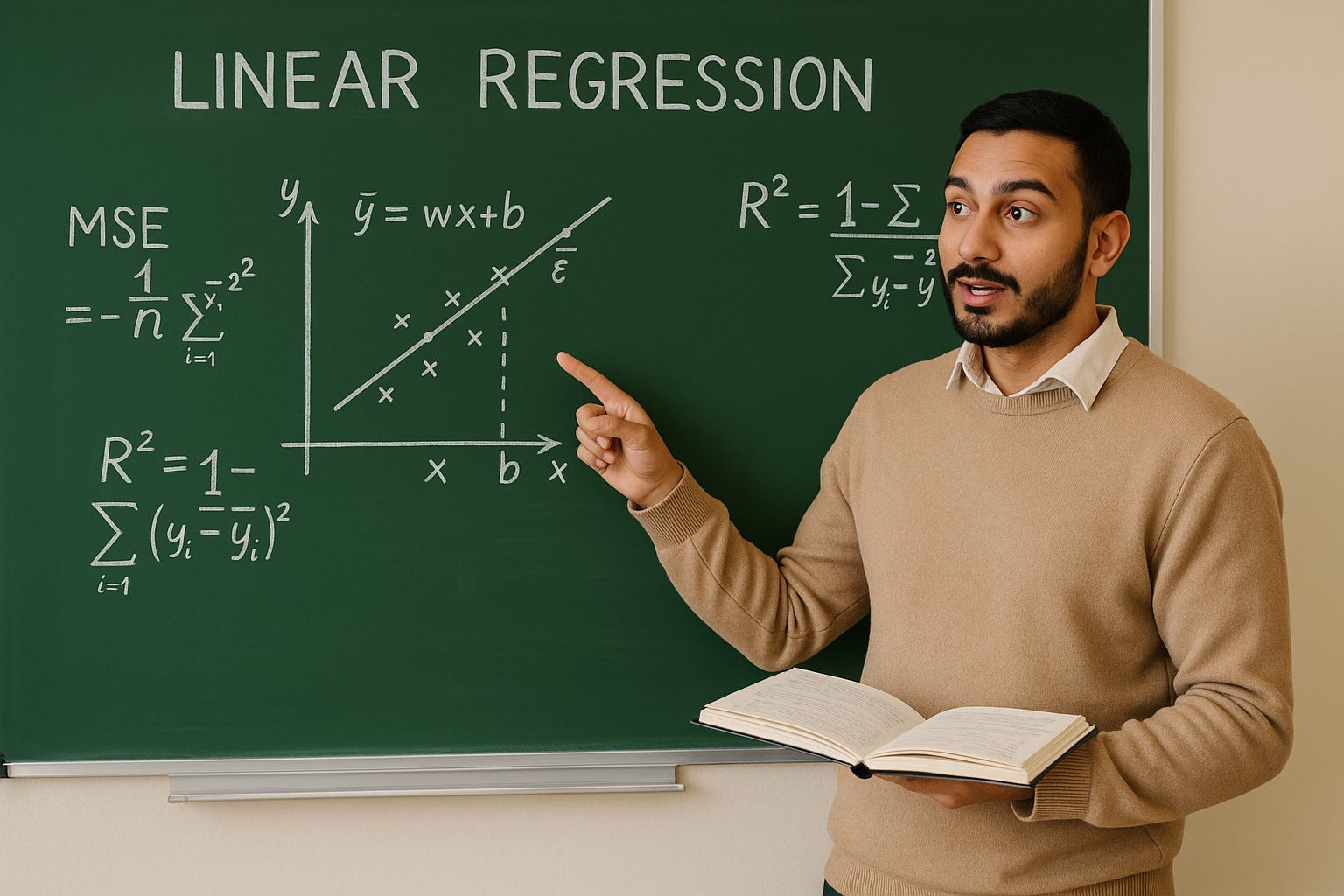
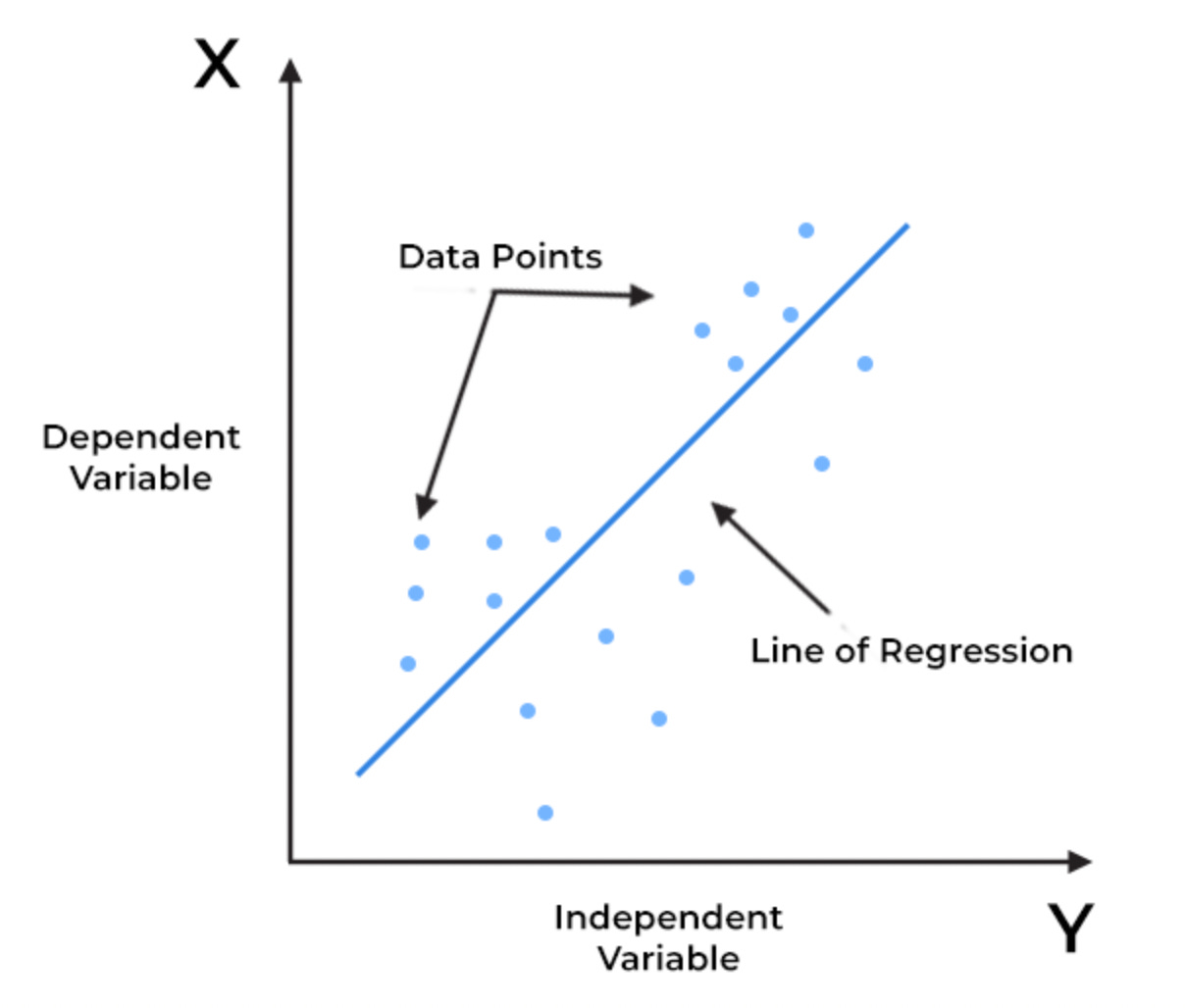
Imagine you're a real estate agent trying to predict the selling price of a house. You notice a trend: larger houses tend to sell for higher prices. How would you quantify this relationship? You might try to draw a straight line through a scatter plot of house size vs. price, aiming to capture the general trend. This "best-fit" line is precisely what Linear Regression seeks to find.
The fundamental goal of Linear Regression is to model the relationship between a dependent variable (the outcome you want to predict, e.g., house price) and one or more independent variables (the features or predictors, e.g., house size) by fitting a linear equation to the observed data.
Why do we use it?
Simplicity and Interpretability: It's easy to understand. The coefficients directly tell you how much the dependent variable is expected to change for a unit increase in an independent variable.
Strong Baseline: Often, even for complex problems, a Linear Regression model provides a surprisingly good baseline performance, against which more complex models can be compared.
Foundation: Understanding Linear Regression is crucial before moving on to more advanced regression or classification techniques.
The core assumption is that there's a linear relationship between your features and the target. If the relationship isn't linear, Linear Regression might not be the best fit, or you might need to transform your features.
🧮 Mathematical Formulation
Simple Linear Regression
The equation for simple linear regression is:
Where:
y: The dependent variable (the value we want to predict, e.g., house price).
x: The independent variable (the feature we use for prediction, e.g., house size).
b: The bias term (or intercept). This is the value of y when x is zero. It represents the baseline value of our prediction.
w: The weight (or slope/coefficient) of the independent variable. It represents how much y is expected to change for every one-unit increase in x. If w is positive, y increases with x; if negative, y decreases.
Multiple Linear Regression
For multiple features, the equation extends to:
Or, in vectorized form:
Where:
Y: A vector of dependent variable values.
X: The feature matrix (or design matrix), where each row represents an observation and each column represents a feature. To handle the bias term b within the matrix multiplication, X is often augmented with a column of ones.
W: A vector of weights (coefficients), where w_j corresponds to the weight for feature X_j.
b: A scalar bias term that is added to all predictions. In a vectorized context, this scalar bias b is added to every prediction.
The above equation represents a hyperplane in a p-dimensional space. For instance, with two features (X1, X2), the model represents a plane in a 3D space, and with more features, it's a hyperplane that we can't visualize directly but conceptually works the same way.
The Cost Function: How Do We Find the 'Best' Line?
How do we determine the "best-fit" line or hyperplane? We need a way to quantify how "bad" our current line is. This is where the cost function (also known as a loss function) comes in. It measures the discrepancy between our model's predictions and the actual observed values.
For Linear Regression, the most common cost function is the Mean Squared Error (MSE).
Mean Squared Error (MSE)
The most commonly used loss function is the Mean Squared Error:
Where:
J(w, b): The cost function, which we want to minimize. It's a function of our model's parameters: weights (w) and bias (b).
m: The total number of training examples.
f(x(i)): The predicted value of y for the i-th training example x(i), given our current w and b values.
y(i): The actual (true) value of y for the i-th training example.
(f(x(i))−y(i)): The error (or residual) for the i-th example.
The sum is the squared errors for all training examples. Squaring the errors does two important things:
It ensures all errors are positive, so positive and negative errors don't cancel each other out.
It heavily penalizes larger errors, pushing the model to reduce them more significantly.
1/2m: This scales the sum. The 1/m averages the squared errors, making the cost function independent of the number of training examples. The 1/2 is a mathematical convenience that simplifies the derivative calculation (it cancels out a 2 from the power rule), making gradient descent updates cleaner, but doesn't change the minimum.
Our goal is simple: find the values of w and b that minimize this MSE cost function.
Solving for the Coefficients: Two Approaches
There are two primary ways to find the optimal weights (w) and bias (b) that minimize the MSE: Gradient Descent (an iterative approach) and the Normal Equation (a closed-form solution).
A. Gradient Descent (Iterative Solution)
Imagine you're standing on a mountain and want to reach the lowest point (the minimum of the cost function). You can't see the whole mountain, but you can feel the slope. You take a small step in the direction of the steepest descent. You repeat this process, taking small steps, until you reach the bottom. That's the intuition behind Gradient Descent.
Algorithm Steps (High-Level):
Initialize Parameters: Start with random (or zero) values for your weights (w) and bias (b).
Calculate Gradients: Compute the partial derivatives of the cost function J(w,b) with respect to each parameter (wj and b). These derivatives tell us the "slope" or direction of the steepest ascent at our current point.
For each weight wj:
\(\frac{\partial}{\partial w_j} J(w,b) = \frac{1}{m} \sum_{i=1}^{m} (h_{w,b}(x^{(i)}) - y^{(i)})x_j^{(i)}\)For bias b:
\(\frac{\partial}{\partial b} J(w,b) = \frac{1}{m} \sum_{i=1}^{m} (h_{w,b}(x^{(i)}) - y^{(i)})\)
Update Parameters: Adjust each parameter in the opposite direction of its gradient (i.e., downhill) by a small amount determined by the learning rate.
Repeat: Continuously repeat steps 2 and 3 for a fixed number of iterations or until the changes in w and b become very small (i.e., convergence).
α (Learning Rate): This hyper-parameter controls the size of the steps you take down the mountain.
Too large α: You might overshoot the minimum and fail to converge, or even diverge.
Too small α: Convergence will be very slow, requiring many iterations.
Advantages:
Scalability: Works well even with very large datasets (m can be huge) and many features (p).
Flexibility: Adaptable to various models and non-convex cost functions (though MSE is convex for Linear Regression).
Disadvantages:
Learning Rate Tuning: Requires careful tuning of the learning rate (α).
Speed: Can be slow if the learning rate is too small or if the dataset is extremely large and computationally expensive to iterate over.
B. Normal Equation (Closed-Form Solution)
Unlike Gradient Descent, which is iterative, the Normal Equation provides a direct, closed-form mathematical solution for the optimal weights and bias. It bypasses the need for iteration or setting a learning rate.
The intuition is that the minimum of the convex MSE cost function occurs where its gradient is zero. By setting the partial derivatives to zero and solving for w and b, we can directly find their optimal values.
The formula for the optimal weights (including the bias term) is:
Where:
W: The optimal vector of weights. This vector will include the bias term b if your design matrix X has been augmented with a column of ones. For an m×p feature matrix, the design matrix X would be m×(p+1) with the first column being all ones, and W would be a (p+1)×1 vector where the first element is the bias b.
X: The design matrix. This matrix is created by taking your feature matrix and adding an extra column of ones to represent the intercept (bias) term. If you have m samples and p features, X will be an m×(p+1) matrix.
Derivation (Brief): The derivation involves setting the gradient of the MSE cost function (in its vector form) with respect to W to zero and then solving for W. This requires some linear algebra manipulations, primarily involving matrix calculus rules.
Advantages:
No Learning Rate: You don't need to choose or tune a learning rate.
Guaranteed Optimal Solution: For Linear Regression, the Normal Equation directly calculates the global minimum of the convex MSE cost function.
Disadvantages:
Computational Expense: Calculating the inverse can be computationally very expensive, especially when the number of features (p) is large. The complexity is roughly O(p^3). For millions of features, this becomes impractical.
Invertibility: (X^TX) must be invertible. This condition might not hold if you have linearly dependent features (multicollinearity) or if the number of features is greater than the number of training examples (p>m).
Regularization: Dealing with Overfitting
Linear Regression, especially with many features, can sometimes suffer from overfitting. This happens when the model learns the training data too well, capturing noise and specific patterns that don't generalize to new, unseen data. Overfitting often manifests as very large weights, making the model overly sensitive to individual data points.
Regularization is a technique used to combat overfitting by adding a penalty term to the cost function. This penalty discourages the model from assigning excessively large weights to features. The intuition is to "regularize" or "constrain" the weights, forcing them to be smaller and promoting a simpler, more generalized model.
A. Ridge Regression (L2 Regularization)
Ridge Regression adds an L2 penalty to the MSE cost function. The L2 penalty is proportional to the sum of the squares of the weights.
Modified Cost Function:
Where:
λ: The regularization parameter. This crucial hyper-parameter controls the strength of the penalty.
If λ=0, Ridge Regression becomes standard Linear Regression.
As λ increases, the penalty on the weights increases, forcing them to shrink closer to zero.
The sum is taken over squared of the weights.
Effect:
Shrinks Weights: Ridge regression shrinks the weights towards zero, but it rarely makes them exactly zero. All features will still contribute to the prediction.
Handles Multicollinearity: It's particularly useful when you have highly correlated features, as it can distribute the weight among them, preventing numerical instability.
B. Lasso Regression (L1 Regularization)
Lasso (Least Absolute Shrinkage and Selection Operator) Regression adds an L1 penalty to the MSE cost function. The L1 penalty is proportional to the sum of the absolute values of the weights.
Modified Cost Function:
Where:
λ: The regularization parameter, similar to Ridge.
The sum is taken over the absolute values of the weights.
Effect:
Feature Selection (Sparsity): The key differentiator of Lasso is its ability to shrink some weights exactly to zero. This effectively performs feature selection, eliminating less important features from the model. This makes the model simpler and more interpretable.
Sparsity: Promotes sparse models where only a subset of features has non-zero weights.
C. Elastic Net Regression
Elastic Net Regression combines both L1 (Lasso) and L2 (Ridge) penalties. It's a compromise that aims to get the best of both worlds.
Formula:
Where:
λ1: Regularization parameter for the L1 (Lasso) penalty.
λ2: Regularization parameter for the L2 (Ridge) penalty.
Advantages:
Combines Benefits: Inherits the regularization strength of Ridge and the feature selection capabilities of Lasso.
Better for Highly Correlated Features: When features are highly correlated, Lasso tends to arbitrarily pick one and zero out the others. Elastic Net can select groups of correlated features, making it more stable.
🛠️ Practical Implementation (Python)
Here’s how you can implement it using scikit-learn:
from sklearn.linear_model import LinearRegression

model = LinearRegression()
model.fit(X_train, y_train)
predictions = model.predict(X_test)
When to Use (and Not Use) Linear Regression
Use Cases:
Simple Predictions: When you need a straightforward model for continuous outcome prediction.
Baseline Models: Often the first model to try, serving as a benchmark for more complex algorithms.
Understanding Relationships: When the primary goal is to understand how changes in independent variables affect the dependent variable.
Situations with Linear Relationships: When domain knowledge or exploratory data analysis suggests a linear association.
Limitations:
Sensitive to Outliers: Outliers can disproportionately influence the "best-fit" line, leading to skewed results.
Assumes Linearity: Cannot inherently capture complex non-linear relationships. Feature engineering (e.g., polynomial features) might be required.
Not for Classification: Designed for continuous outcomes; for categorical outcomes, logistic regression or other classification algorithms are used.
Doesn't Perform Feature Scaling Automatically: While not a strict limitation, performance can sometimes improve with feature scaling, especially for Gradient Descent.
10 Frequently Asked Linear Regression Interview Questions
Beyond understanding the theory, data science interviews often test your grasp of practical implications and common pitfalls. Here are 10 frequently asked questions related to Linear Regression, designed to solidify your knowledge for interviews:
1. What are the core assumptions of Linear Regression, and why are they important?
Assumptions:
Linear relationship between features and the target.
Independent observations and errors.
Errors are normally distributed with constant variance (homoscedasticity).
Minimal multicollinearity among independent variables.
Importance:
Violations can lead to biased or inefficient coefficient estimates.
They can result in inaccurate p-values and confidence intervals.
Ultimately, this compromises model interpretability and reliability.
2. Explain the difference between Simple Linear Regression and Multiple Linear Regression.
Simple Linear Regression (SLR):
Uses one independent variable to predict a continuous dependent variable.
Fits a straight line to the data, showing how a single factor influences the outcome.
Multiple Linear Regression (MLR):
Uses two or more independent variables to predict a continuous dependent variable.
Fits a hyperplane in higher dimensions, analyzing how multiple factors jointly influence the outcome.
3. What is the Mean Squared Error (MSE) and why is it commonly used as the cost function for Linear Regression?
What it is:
MSE quantifies the average of the squared differences between predicted and actual values.
Why used:
It's a convex function, guaranteeing a single global minimum, which simplifies optimization.
By squaring errors, it heavily penalizes larger deviations, promoting more accurate predictions.
4. Differentiate between Gradient Descent and the Normal Equation for solving Linear Regression.
Gradient Descent:
An iterative optimization algorithm that gradually adjusts parameters towards the minimum cost.
Requires tuning a learning rate.
Normal Equation:
A direct, closed-form analytical solution that calculates optimal parameters in one step.
Does not require iteration or a learning rate.
5. When would you prefer Gradient Descent over the Normal Equation, and vice-versa?
Gradient Descent preferred when:
Dealing with very large datasets or a high number of features (computationally more feasible).
Suitable for online learning or when data doesn't fit into memory.
Normal Equation preferred when:
Working with smaller datasets or a limited number of features (faster and guarantees optimum).
No need for learning rate tuning.
6. Explain the concept of multicollinearity in Linear Regression. How can it be detected and what are its consequences?
Concept:
Occurs when independent variables are highly linearly correlated with each other.
Detection:
Examine correlation matrices or calculate Variance Inflation Factor (VIF).
Consequences:
Leads to unstable and unreliable coefficient estimates.
Makes it difficult to interpret individual feature importance.
Doesn't necessarily affect overall predictive power, but harms interpretability.
7. What is regularization in Linear Regression, and why is it used?
What it is:
A technique to prevent overfitting by adding a penalty term to the cost function.
Why used:
Discourages assigning excessively large weights to features.
Forces the model to learn simpler, more robust patterns.
Improves generalization to unseen data.
8. Differentiate between Ridge and Lasso Regression.
Ridge (L2) Regression:
Adds a penalty proportional to the sum of squared weights.
Shrinks weights towards zero but rarely to exactly zero.
Effective for handling multicollinearity.
Lasso (L1) Regression:
Adds a penalty proportional to the sum of the absolute values of weights.
Can shrink some weights precisely to zero, performing automatic feature selection.
9. When would you use Elastic Net Regression?
Use Case:
When you want to combine the benefits of both Ridge and Lasso regularization.
Ideal for datasets with many features, especially if some are highly correlated.
Provides both group selection for correlated features (like Ridge) and sparsity (feature elimination, like Lasso).
10. What are the limitations of Linear Regression, and when might you choose a different model?
Limitations:
Assumes a linear relationship, struggling with inherently non-linear patterns.
Sensitive to outliers, which can significantly skew the model's fit.
Designed for continuous targets; not suitable for classification.
When to choose other models:
For complex non-linear relationships (e.g., polynomial regression, decision trees, neural networks).
For categorical outcomes (e.g., logistic regression).
When data has severe outliers that cannot be addressed.
Conclusion
Linear Regression stands as a cornerstone of machine learning, offering a transparent and interpretable approach to prediction. From its intuitive goal of finding the best-fit line to its robust mathematical foundations and advanced regularization techniques, it provides a solid starting point for any data scientist.
What are your thoughts on Linear Regression? Have you used it in interesting projects? Share your experiences in the comments below! Follow me for more insights into the fascinating world of machine learning.
Support My Work
If you found this post valuable, consider supporting my work with a small contribution via UPI. Your support:
Helps me and my team spend more time simplifying complex ML topics
Keeps deep-dive content accessible to everyone
Fuels more research and better-quality posts
UPI ID: manishmazumder-1@okaxis (scan below QR!)
Thank you for being part of this learning journey!

Thanks for the post, very informative, detailed from intuition till implementation
Anticipating more such posts regarding other algorithms in-depth
:)