XGBoost Explained: The “Extreme” Machine Learning Powerhouse

Imagine gathering a crowd of experts and asking them to predict tomorrow’s stock price. Each expert gives an independent opinion, and you average their answers—that’s the wisdom of crowds. Random Forests harness this idea beautifully, where each tree votes independently, and the majority decides the outcome.

But what if our experts didn’t just vote on their own… but actually learned from each other’s mistakes? What if each new expert focused precisely on correcting where previous experts went wrong?

Welcome to the world of Boosting—and, more specifically, the mighty XGBoost.

XGBoost is one of the most powerful and widely-used machine learning algorithms today. It’s the engine behind countless Kaggle competition wins and real-world solutions in finance, healthcare, marketing, and more. Built upon the concept of Gradient Boosting, XGBoost adds powerful optimizations and regularization that make it both fast and accurate, especially for tabular (structured) data.

In this guide, we’ll demystify:

• The core idea of Boosting

• How Gradient Boosting works under the hood

• What makes XGBoost truly “extreme”

• Key parameters and how to tune them

• Coding examples

• Strengths and weaknesses of XGBoost

• When (and when not) to use it

Let’s dive in!

The Intuition: Learning from Mistakes (Boosting vs. Bagging)

Picture a student learning math. On the first try, they solve some problems but make mistakes. Next, they carefully review their errors and focus only on those problem areas. Each new study session corrects the errors of the last, bringing them closer to mastery.

Boosting works the same way.

• Boosting is an ensemble technique that builds models sequentially. Each new model tries to correct the mistakes made by the combined previous models.

• Contrast this with Bagging (used in Random Forests):

  • Bagging grows many trees in parallel, each independently trained on random samples of data and features. Predictions are combined via averaging (regression) or majority vote (classification).

  • Goal: reduce variance by creating many independent, diverse models.

In Boosting, models are dependent:

• Each tree sees the errors left by the trees before it.

• The ensemble focuses on reducing bias by continually improving on its weaknesses.

This is why boosting algorithms often achieve higher accuracy than bagging—at the cost of more complexity and potential overfitting if not carefully tuned.

---

From Boosting to Gradient Boosting

The Early Idea: AdaBoost

In classic boosting (like AdaBoost), misclassified samples get higher weights for the next model, forcing subsequent trees to focus on “hard” examples.

However, AdaBoost has some limitations, especially with noisy data and certain loss functions.

---

Enter Gradient Boosting

Instead of simply reweighting samples, Gradient Boosting takes a more elegant route:

• Rather than predicting the target directly, each new tree predicts the residuals (the mistakes) of the current ensemble’s predictions.

In other words:

Each new tree answers the question: “What’s left to explain?”

This process is akin to gradient descent, an optimization technique used across machine learning:

• Gradient descent finds the direction in which to adjust parameters to minimize a loss function.

• Gradient Boosting does the same—each new tree represents a step in the direction that reduces the loss the most.

Mathematically, if your current prediction is:

\(\hat{y}_i^{(m-1)} \)

Then the residual for sample i is:

\(r_i^{(m)} = y_i - \hat{y}_i^{(m-1)}\)

The next tree is trained on these residuals.

It’s called Gradient Boosting because it uses gradient descent to minimize a loss function. Just like neural networks adjust weights to reduce loss, gradient boosting adjusts trees.

Suppose your loss function is L(y, y_hat). Gradient Boosting takes a step in the negative gradient direction:

\(r_i^{(m)} = -\left[ \frac{\partial L(y_i, \hat{y}_i^{(m-1)})}{\partial \hat{y}_i^{(m-1)}} \right]\)

Each tree learns to push predictions closer to the target by moving in the steepest descent direction of the loss curve.

Key Point: Gradient Boosting converts boosting into an optimization problem solved via gradients.

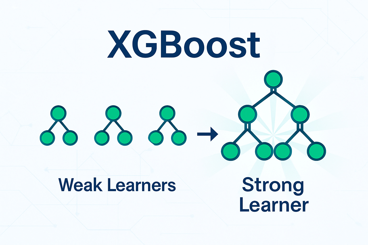
Weak Learners: These trees are usually shallow (small depth). Individually, they’re weak models. Together, they’re incredibly strong.

---

What Makes XGBoost “Extreme”? (Beyond Standard Gradient Boosting)

XGBoost isn’t just another Gradient Boosting implementation. It’s famous for being:

• Faster

• More scalable

• Better regularized

• Highly customizable

Let’s unpack what makes it so special.

---

What Makes XGBoost “Extreme”? (Beyond Standard Gradient Boosting)

Gradient Boosting is powerful — but XGBoost takes it to a whole new level with:

✅ Regularization
✅ System-level optimizations
✅ Algorithmic tricks for speed & scalability

Let’s unpack why it’s “Extreme.”

---

Regularization

Ordinary gradient boosting can easily overfit. XGBoost introduces regularization directly into its objective.

Its regularized objective looks like this:

\(\text{Obj} = \sum_{i=1}^n L(y_i, \hat{y}_i) + \sum_{k=1}^{K} \Omega(f_k)\)

where:

\(\Omega(f_k) = \gamma T + \frac{1}{2} \lambda \sum_{j=1}^{T} w_j^2\)

• T = number of leaves in the tree

• w_j​ = leaf weights

• γ = cost of adding a new leaf

• λ = L2 regularization term

XGBoost also supports L1 regularization via the parameter reg_alpha.

Regularization controls tree complexity and reduces overfitting.

---

Shrinkage (Learning Rate)

After each tree’s contribution, XGBoost scales its impact:

\(\hat{y}_i^{(m)} = \hat{y}_i^{(m-1)} + \eta \cdot f_m(x_i)\)

• η = learning rate (typically 0.01–0.3)

Smaller learning rates make the model more robust but require more trees.

---

Column (Feature) Subsampling

Like Random Forests, XGBoost can randomly sample features:

• colsample_bytree = fraction of features used by each tree

• Helps reduce correlation between trees

• Improves generalization

---

Tree Pruning

XGBoost uses a clever pruning strategy:

• Starts building trees fully

• Prunes branches where the gain is below a threshold

• Reduces over-complex trees

---

System-Level Optimizations

Parallelization

While boosting overall is sequential, tree construction in XGBoost is parallelized:

• Finds the best split across all features simultaneously.

---

Approximate Tree Learning

For massive datasets, XGBoost uses techniques like:

• Quantile sketches to approximate split points quickly.

• Greatly speeds up training without major accuracy loss.

---

Cache-aware Computation

XGBoost optimizes how data is stored and accessed to maximize CPU cache usage, reducing memory bottlenecks.

---

Out-of-Core Computing

When data doesn’t fit into memory, XGBoost processes it in manageable chunks.

---

Flexibility

• Custom Loss Functions: Users can define custom objectives for specialized tasks.

• Built-in Cross-Validation: Cross-validation can run during training.

• Handling Missing Values: XGBoost automatically learns the optimal way to send missing values left or right in a split based on minimizing loss.

This unique blend of robust regularization and blazing-fast system design is why XGBoost became a powerhouse for ML competitions and industry applications.

---

Key Parameters in XGBoost (Briefly)

Here’s a quick cheat sheet for tuning XGBoost:

• n_estimators (or num_boost_round)
  Number of boosting rounds (trees).

• learning_rate
  Shrinkage factor for each tree’s contribution.

• max_depth
  Maximum depth of trees.

• subsample
  Fraction of training samples used per tree.

• colsample_bytree
  Fraction of features sampled per tree.

• objective
  Loss function to minimize (e.g. 'reg:squarederror', 'binary:logistic').

• reg_alpha (L1) & reg_lambda (L2)
  Regularization terms for controlling model complexity.

---

1. Random Forest vs. XGBoost (Regression Comparison)

import numpy as np
import pandas as pd
from sklearn.datasets import load_boston
from sklearn.model_selection import train_test_split
from sklearn.ensemble import RandomForestRegressor
from xgboost import XGBRegressor
from sklearn.metrics import mean_squared_error

# Load sample data
boston = load_boston()
X = boston.data
y = boston.target

X_train, X_test, y_train, y_test = train_test_split(X, y, test_size=0.2, random_state=42)

# Random Forest
rf = RandomForestRegressor(n_estimators=100, random_state=42)
rf.fit(X_train, y_train)
rf_preds = rf.predict(X_test)
rf_rmse = mean_squared_error(y_test, rf_preds, squared=False)

# XGBoost
xgb = XGBRegressor(n_estimators=100, random_state=42)
xgb.fit(X_train, y_train)
xgb_preds = xgb.predict(X_test)
xgb_rmse = mean_squared_error(y_test, xgb_preds, squared=False)

print(f"Random Forest RMSE: {rf_rmse:.4f}")
print(f"XGBoost RMSE: {xgb_rmse:.4f}")

---

2. XGBoost Regression Example

from xgboost import XGBRegressor
from sklearn.datasets import make_regression
from sklearn.model_selection import train_test_split
from sklearn.metrics import mean_squared_error

# Generate synthetic data
X, y = make_regression(n_samples=1000, n_features=10, noise=0.3, random_state=42)

# Train/test split
X_train, X_test, y_train, y_test = train_test_split(X, y, test_size=0.2, random_state=42)

# Create and fit XGBoost model
model = XGBRegressor(n_estimators=100, learning_rate=0.1, max_depth=3, random_state=42)
model.fit(X_train, y_train)

# Predictions
y_pred = model.predict(X_test)
rmse = mean_squared_error(y_test, y_pred, squared=False)
print(f"RMSE: {rmse:.4f}")

---

3. XGBoost Classification Example

from xgboost import XGBClassifier
from sklearn.datasets import make_classification
from sklearn.model_selection import train_test_split
from sklearn.metrics import accuracy_score

# Create binary classification data
X, y = make_classification(n_samples=1000, n_features=20, random_state=42)

X_train, X_test, y_train, y_test = train_test_split(X, y, test_size=0.2, random_state=42)

# Fit XGBoost classifier
clf = XGBClassifier(n_estimators=100, learning_rate=0.1, max_depth=3, random_state=42)
clf.fit(X_train, y_train)

# Evaluate
y_pred = clf.predict(X_test)
acc = accuracy_score(y_test, y_pred)
print(f"Accuracy: {acc:.4f}")

---

4. Plotting Feature Importance

import matplotlib.pyplot as plt
from xgboost import plot_importance

# Assuming model is an XGBRegressor or XGBClassifier
plot_importance(model)
plt.show()

This helps visualize which features contribute most to your predictions.

---

5. Hyperparameter Tuning Example

from sklearn.model_selection import GridSearchCV
from xgboost import XGBRegressor

param_grid = {
    "max_depth": [3, 5, 7],
    "learning_rate": [0.01, 0.1],
    "n_estimators": [50, 100, 200],
}

grid = GridSearchCV(
    estimator=XGBRegressor(random_state=42),
    param_grid=param_grid,
    scoring="neg_mean_squared_error",
    cv=3,
    verbose=1
)

grid.fit(X_train, y_train)
print("Best parameters:", grid.best_params_)
print("Best score:", -grid.best_score_)

---

Strengths of XGBoost

✅ High Performance/Accuracy
Especially strong on structured/tabular data.

✅ Speed and Scalability
Highly optimized implementation.

✅ Robust to Overfitting
Thanks to regularization and shrinkage.

✅ Handles Missing Values
No need to impute missing data manually.

✅ Flexibility
Custom losses and metrics.

✅ Feature Importance
Helpful insights into what drives predictions.

---

Weaknesses of XGBoost

❌ Less Interpretable
An ensemble of many trees = black box.

❌ Sensitive to Hyperparameters
Requires careful tuning.

❌ Sequential Nature
Boosting is fundamentally sequential (limits distributed training).

❌ Prone to Overfitting if Not Tuned
Its power is a double-edged sword.

❌ Memory Intensive
Especially with deep trees or many estimators.

---

When to Use (and Not Use) XGBoost

✅ Use XGBoost When:

• You need top-tier accuracy on tabular data.

• Your dataset is large and structured.

• You want feature importance insights.

• Kaggle competitions or high-stakes applications demand maximum predictive power.

🚫 Avoid XGBoost When:

• Model interpretability is critical (e.g. legal, healthcare decisions).

• You have a very small dataset (risk of overfitting).

• Your data is unstructured (images, text) and better served by deep learning.

• You’re severely constrained on memory resources.

---

Conclusion: The King of Tabular Data?

XGBoost isn’t just another algorithm—it’s a highly-tuned engine for predictive accuracy. By combining sequential learning with ruthless optimization, it’s earned its reputation as a competition killer.

Still, it’s not the only game in town. Other powerful gradient boosting libraries like LightGBM and CatBoost offer competitive speed and unique strengths worth exploring.

Next Steps:

1. Try it on a Kaggle dataset (e.g., Titanic, House Prices).

2. Compare it to Random Forests—when does it win?

3. Explore siblings like LightGBM (faster) or CatBoost (handles categories natively).

Follow me for more intuitive ML deep dives and powerful algorithm breakdowns!